2 Low-level image statistics in natural scenes influence perceptual decision-making

Abstract A fundamental component of interacting with our environment is gathering and interpretation of sensory information. When investigating how perceptual information influences decision-making, most researchers have relied on manipulated or unnatural information as perceptual input, resulting in findings that may not generalize to real-world scenes. Unlike simplified, artificial stimuli, real-world scenes contain low-level regularities that are informative about the structural complexity, which the brain could exploit. In this study, participants performed an animal detection task on low, medium or high complexity scenes as determined by two biologically plausible natural scene statistics, contrast energy (CE) or spatial coherence (SC). In experiment 1, stimuli were sampled such that CE and SC both influenced scene complexity. Diffusion modeling showed that both the speed of information processing and the required evidence were affected by low-level scene complexity. Experiment 2a/b refined these observations by showing how isolated manipulation of SC resulted in weaker but comparable effects, whereas manipulation of only CE had no effect. Overall, performance was best for scenes with intermediate complexity. Our systematic definition quantifies how natural scene complexity interacts with decision-making. We speculate that CE and SC serve as an indication to adjust perceptual decision-making based on the complexity of the input.

This chapter is published as: Seijdel, N., Jahfari, S., Groen, I.I.A. & Scholte, H.S. (2020). Low-level image statistics in natural scenes influence perceptual decision-making. Scientific Reports 10, 10573. https://doi.org/10.1038/s41598-020-67661-8

2.1 Introduction

During decision-making, observers extract meaningful information from the sensory environment in a limited amount of time. In recent computational accounts of perceptual decision-making, sensory evidence for a decision option is integrated and accumulates over time until it reaches a certain boundary (Gold & Shadlen, 2007; Heekeren et al., 2008). Across these computational accounts, the speed of evidence accumulation is thought to depend on the quality or strength of sensory information available (the drift rate, as formalized with the well-known drift diffusion model (Ratcliff & McKoon, 2008).

In the current study, we aimed to investigate how decision-making processes are influenced by low-level image properties, diagnostic of scene complexity. While multiple studies have shown that specific image properties (such as spatial frequency, or stimulus strength) interact with decision-making, they manipulate visual information into “unnatural” stimuli. For example, we recently showed that image quality modulates response inhibition, and decision-making processes (Jahfari et al., 2015), by manipulating the spatial frequencies of images. Ultimately, however, our goal is to understand how decision processes are influenced by information in natural scenes (Malcolm et al., 2016). The scenes that we encounter in our everyday environment do not contain randomly sampled pixels, but adhere to specific low-level regularities called natural scene statistics. Natural scene statistics have been demonstrated to carry diagnostic information about the visual environment: for example, slopes of spatial frequency spectra estimated across different spatial scales and orientations (‘spectral signatures’) are informative of scene category and spatial layout (Greene & Oliva, 2009b, 2009a; Oliva & Torralba, 2001). Similarly, the width and shape of histograms of local edge information estimated using single- and multi-scale non-oriented contrast filters have been shown to systematically differ with scene category and complexity (Brady & Field, 2000; Ghebreab et al., 2009; Scholte et al., 2009).

Earlier studies have shown that visual activity evoked by natural scenes can be well described by scene complexity, suggesting that the brain is adapted or tuned to those statistical regularities (Ghebreab et al., 2009; Scholte et al., 2009), and potentially using them during visual perception. Scene complexity reflected in local contrast distributions can be estimated using an early visual receptive field model that outputs two parameters, contrast energy (CE) and spatial coherence (SC), approximating the scale and shape of a Weibull fit to the local contrast distribution, respectively (see Supplementary section 1). CE and SC reflect different aspects of the local contrast distribution: CE approximates the scale parameter of the Weibull fit and reflects the average local contrast strength in an image. SC approximates the shape parameter of the Weibull fit and reflects to what degree the contrast distribution resembles a power law or Gaussian distribution. Cluttered or complex scenes, with high CE/SC values, have more Gaussian (bell-shaped) distributions compared to sparse or simple scenes with low CE/SC values (power-law shaped), that often contain one or a few salient objects (Figure 2.1; adapted from Groen et al. (2013)).

Importantly, CE and SC are computed using a simple visual model that simulates neuronal responses in one of the earliest stages of visual processing. Specifically, they are derived by averaging the simulated population response of LGN-like contrast filters across the visual scene (Scholte et al., 2009). Similar to other models of representation in early vision (e.g. Rosenholtz et al. (2012)), these two-parameters thus provide a compressed representation of a scene. In turn, they could serve as a complexity index that affects subsequent computations towards a task-relevant visual representation.

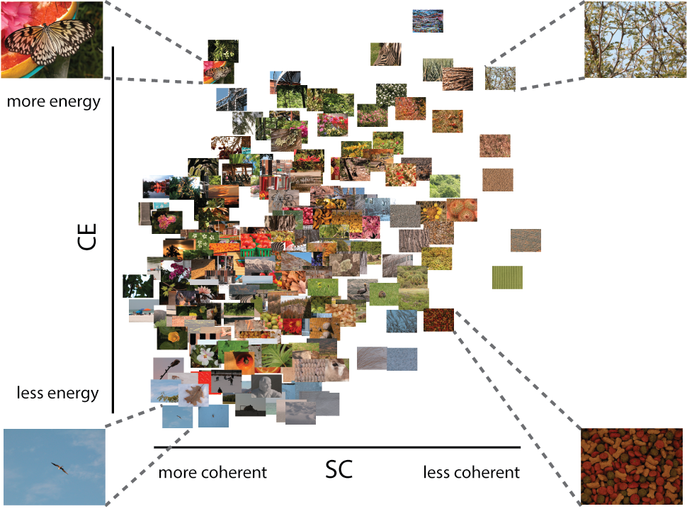
Figure 2.1: (ref:caption-figure-scenestats-stim)

(ref:caption-figure-scenestats-stim) A Subselection of stimuli plotted against their CE and SC values. Figure adapted from Groen et al. (2013). SC (the approximation of the \(\gamma\) parameter of the Weibull function) describes the shape of the contrast distribution: it varies with the amount of scene fragmentation (scene clutter). CE (the approximation of the \(\beta\) parameter of the Weibull function) describes the scale of the contrast distribution: it varies with the distribution of local contrasts strengths. Four representative pictures are shown in each corner of the parameter space. Images that are highly structured (e.g., a street corner) are found on the left, whereas highly cluttered images (e.g., a forest) are on the right. Images with higher figure-ground separation (depth) are located on the top, whereas flat images are found at the bottom.

Here, we investigated whether task-irrelevant manipulations of SC and CE interact with perceptual decision-making by using the drift-diffusion model (DDM). By considering response time distributions for both correct and incorrect choices, the DDM models the speed of evidence accumulation, as well as the amount of evidence required to make a decision. In experiment 1, stimuli were selected such that both CE and SC co-varied with scene complexity, with increasing values representing more complex natural scenes. This is the ‘natural situation’, since SC and CE are typically correlated within our natural environment. To refine the observations in experiment 1, in experiment 2a and 2b, we also selected stimuli in such a way that the effects for both parameters could be evaluated separately.

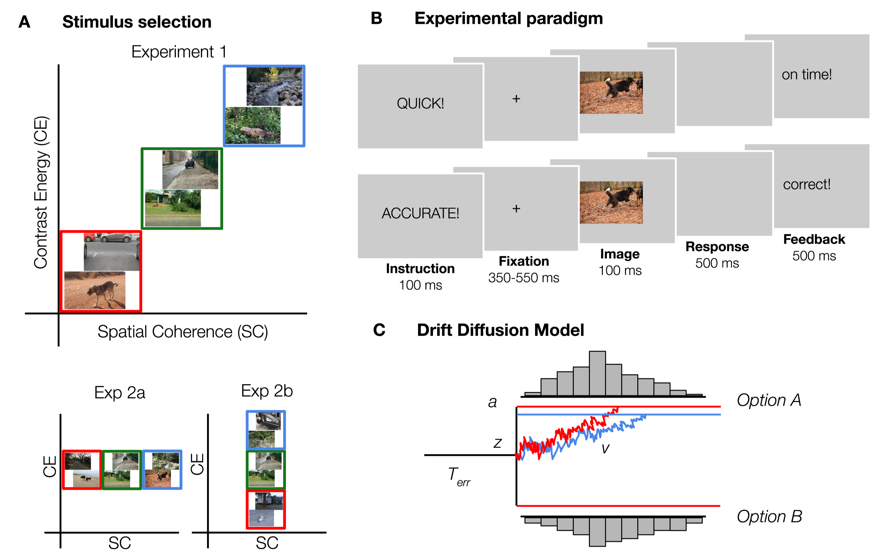
Figure 2.2: Experimental design and methods. A) Examples of the stimuli used in experiment 1, 2a and 2b. Images varied both in SC and CE (red = low, green = medium, blue = high) in experiment 1. To investigate whether it is meaningful to differentiate between SC and CE, the two parameters were manipulated separately in experiments 2a (SC) and 2b (CE). For each condition, 80 animal and non-animal scenes were selected. B) Experimental paradigm. Participants categorized scenes based on the presence or absence of an animal. On half of the trials, participants were asked to respond as quickly as possible (“speed trials”), as indicated by a pre-cue. On the other half of the trials, participants had to respond as accurate as possible (“accurate trials”). C) Schematic representation of the Drift Diffusion Model. From a starting point \(z\), information begins to accumulate in favor of one of the options with drift rate \(v\) until it reaches a boundary \(a\), and the decision is made. Non-decision time \(Terr\) captures the processes that are unrelated to decision-making, such as response execution.

2.2 Materials and methods

2.2.1 Experiment 1

In experiment 1, we investigated the combined influence of SC and CE on decision-making. As SC and CE are generally highly correlated, varying them together provides the strongest manipulation of information. We expected the drift rate to decrease with increased scene complexity, with an additional shift in the amount of evidence required (boundary) reflecting potential strategic adjustments to the complexity of the scene.

2.2.1.1 Participants

Twenty participants (7 males) aged between 18 and 25 years (M = 21.9, SD = 1.9) with normal or corrected-to-normal vision, gave written informed consent prior to participation and were rewarded with research credits or monetary compensation. The ethics committee of the University of Amsterdam approved the experiment. All experimental protocols and methods described below were carried out in accordance with the guidelines and regulations of the University of Amsterdam.

2.2.1.2 Stimuli

480 images (640*480 pixels, full-color) were obtained from a previous study by Groen et al. (2010). The complete image set contained 7200 scenes from online databases, including the INRIA holiday database (Jegou et al., 2008), the GRAZ database (Opelt et al., 2006), ImageNet (Deng et al., 2009) and the McGill Calibrated Color Image Database (Olmos & Kingdom, 2004). For each scene, we computed CE and SC values using the model described in Ghebreab et al. (2009) and Groen et al. (2013), and selectively sampled scenes for three conditions: low, medium and high (Figure 2.2). Each condition contained 160 scenes, half of which contained an animal. Importantly, within conditions, animal and non-animal scenes were matched in CE and SC values such that these two categories did not differ from each other in mean or median values (mean: all t(158) < 1.14, all p > 0.26, median: all z < 1.08, all p > 0.28).

2.2.1.3 Procedure

Participants performed an animal/non-animal categorization task (Thorpe et al., 1996) (Figure 2.2). Scenes were presented in randomized sequence, for a duration of 100 ms. Between trials, a fixation-cross was presented with a semi-randomly duration (350, 400, 450, 500 or 550 ms), averaging to 450 ms. There were two trial instructions, that appeared on screen before every trial in randomly alternating blocks of 20 trials: on “speed trials”, participants were asked to respond as fast as possible, whereas on “accuracy trials”, they responded as accurately as they could. While instruction influences both the accuracy and duration of decisions, the ease of evidence accumulation (drift rate) should remain constant (Ratcliff, 2014). Using a Speed-Accuracy manipulation allows for a stronger and more sensitive test of the influence of scene complexity on perceptual decision-making. If animal detection in more complex scenes is indeed associated with more cautious or elaborate processing, performance in the high condition should be most affected for “speed trials, in which extensive visual processing is potentially limited by time constraints. Therefore, we aimed to specify how the processing of natural scenes can modulate decision-making processes when participants emphasize accuracy - and allow ample time for processing - or speed. Every scene was presented once for both instructions (960 trials in total). Keyboard buttons were switched halfway (based on a simultaneous EEG study). Comparing % errors in blocks before and after the switch did not indicate switch costs: Mbefore = 0.13, SD = 0.15; Mafter = 0.16, SD = 0.11, only taking participants into account for which the same instruction was repeated before and after the switch, averaged across experiments. On speed trials, participants received feedback on their response time (”on time" < 500 ms > “too slow”). On accuracy trials, participants were presented with “correct” and “incorrect” feedback. When participants didn’t respond, “miss” appeared on screen. Participants were seated ~90 cm from the monitor such that stimuli subtended ~10x14\(^{\circ}\) of visual angle. Images were presented at eye-level on a 23-inch Asus LCD display (sRGB, 2.27 gamma, 1.31 dE) with a spatial resolution of 1080*1920 pixels, at a refresh rate of 60Hz, using Presentation (version 17.0, Neurobehavioral Systems, Inc.). The ambient illumination in the room was kept constant across different participants.

2.2.1.4 Hierarchical Drift Diffusion Model

We fitted a hierarchical version of the DDM (HDDM; Wiecki et al. (2013)) using the RT distributions of correct and incorrect responses. HDDM uses a hierarchical Bayesian estimation, that uses MCMC sampling to estimate the joint posterior distribution of all model parameters, and has been described as method of preference in estimating drift rates for a small number of observations (in the order of 100-20; Ratcliff & Childers (2015)). HDDM assumes that during decision-making, information begins to accumulate from a starting point \(z\), in favor of one of the options with drift rate \(v\) until it reaches a boundary \(a\), and the decision is made. Non-decision time \(Terr\) captures the processes that are unrelated to the decision-making, such as response execution. (Figure 2.2).

First, we evaluated five models in which drift rate (\(v\)) and boundary (\(a\)) were either fixed or varied across trial type (speed, accurate) and/or scene complexity (low, medium, high). Using the Deviance Information Criterion (DIC) for model selection we established that, next to varying response boundary across trial type (\(\Delta\)DIC = -3404 compared to fixed), varying both parameters across scene complexity was justified to account for the data (Spiegelhalter et al., 2002). This fit produced lower DIC values compared to a fit in which the drift rate (\(\Delta\)DIC = -133.3), response boundary (\(\Delta\)DIC = -40.4) or both (\(\Delta\)DIC = -68.1) were fixed across complexity. Then, to assess the trial-by-trial relationship between scene complexity and drift rate (\(v\)) and boundary separation (\(a\)), we fitted eighteen alternative regression models. Both linear models (SC/CE centered around zero), and second-order polynomial models (quadratic) were fitted to examine whether the relationship was curvilinear (e.g. followed an inverted U-shape). We never included both scene statistics simultaneously, as their high correlation leads to multicollinearity and unstable coefficient estimates. To take into account the effect of task instruction on the response boundary a, we estimated two intercepts for this parameter (speed and accuracy) using the depends_on key argument. For each model, we ran four separate chains with 5,000 samples. The first 200 samples were discarded (burn), resulting in a trace of 19200 samples. Models were tested for convergence using visual inspection of the group level chains and the Gelman-Rubin statistic, which compares the intra-chain variance of the model to the intra-chain variance of the different runs. It was checked that all group-level parameters had an Rhat between 0.98-1.02. For the best fitting model (lowest DIC), we ran posterior predictive checks by averaging 500 simulations generated from the model’s posterior to confirm it could reliably reproduce patterns in the observed data. Bayesian hypothesis testing was performed on the group-level posterior densities for means of parameters. The probability measure P was obtained by calculating the percentage of the posterior < 0 (see Supplementary section 2).

2.2.2 Experiment 2

A key question is whether the effects found in experiment 1 are driven by the two scene statistics together, as they are generally highly correlated in our natural environment, or whether one of them is the primary cause, as suggested by the SC preference in our optimal HDDM model. To refine our interpretation, we systematically manipulated SC while keeping CE constant (experiment 2a) and vice versa (experiment 2b). Experimental procedure and analyses occurred as in experiment 1, except where otherwise indicated.

2.2.2.1 Participants

Twenty-four participants (4 males; aged 18-28 years, M = 21.8, SD = 2.7) participated in experiment 2a; Twenty-seven participants (7 males; aged 18-27 years, M = 21.4, SD = 2.5) participated in experiment 2b. All participants gave written informed consent prior to participation and were rewarded with research credits or monetary compensation. The ethics committee of the University of Amsterdam approved the experiment, and all experimental protocols and methods described below were carried out in accordance with the guidelines and regulations.

2.2.2.2 Stimuli

A new selection of 480 scenes was composed from the same image set as in experiment 1, except that each condition was now defined by either its SC (experiment 2a) or its CE (experiment 2b) values while the other was kept constant at intermediate values (Figure 2.2).

2.2.2.3 Hierarchical Drift Diffusion Model

In experiment 2a we established that, next to varying response boundary across trial type (\(\Delta\)DIC = -3426 compared to fixed), varying both parameters across SC was justified to account for the data. This fit produced lower DIC values compared to a fit in which the drift rate (\(\Delta\)DIC = -70.5), response boundary (\(\Delta\)DIC = -60.3) or both (\(\Delta\)DIC = -27.8) were fixed across complexity. Next, we evaluated nine regression models to assess the trial-by-trial relationship between scene complexity (indexed solely by SC), and drift rate and response boundary. For experiment 2b model selection indicated that a model in which, apart from varying response boundary across trial type, the parameters were fixed across CE best explained the observed data. This fit produced lower DIC values compared to a fit in which the drift rate (\(\Delta\)DIC = -44.7), response boundary (\(\Delta\)DIC = -76.7) or both (\(\Delta\)DIC = -48.5) were allowed to vary across complexity. Thus, variability in CE alone seems to have no influence on the speed of evidence accumulation or the amount of information required to make a decision. As such, further regression analyses were not justified.

2.2.3 Data and code availability

Data and code to reproduce the analyses are available at the Open Science Framework (https://doi.org/10.17605/OSF.IO/J2AB9) and at https://github.com/noorseijdel/2019_scenestats.

2.3 Results

2.3.1 Experiment 1

Data from one participant were excluded for excessive errors (>23%, 2.8 SD > mean). RTs <100 ms were considered “fast guesses” and removed. The repeated-measures ANOVA on RT (on correct trials) revealed main effects of both instruction (speed, accurate) and scene complexity (low, medium, high), but no interaction effect, F(36) = 0.261, p > 0.77. Similarly, the repeated-measures ANOVA on error rates revealed main effects but no interaction effect, F(36) = 0.177, p > 0.83. As expected, responses were faster and less accurate when given a “speed” instruction, in comparison to “accurate”. Because there was no interaction, RTs and error rates were collapsed over speed and accurate trials to further understand how scene complexity modulates decision-making. Bonferroni correction was used for all comparisons.

A repeated-measures ANOVA, with factor scene complexity differentiated RTs across the three conditions, F(2,36) = 19.81, p < .001, \(\eta^{2par}\) = .524 (Figure 2.3. Participants responded slower for high (complex) scenes than for medium-, t(18) = -7.293, p < .001, and low scenes, t(18) = -3.914, p = .001. There was also a main effect on error rates, F(2, 36) = 14.26, p < .001, \(\eta^{2par}\) = .442. Participants made more errors for high scenes than for medium, t(18) = -4.493, p < .001, and low scenes, t(18) = -2.752, p = .013. Remarkably, participants made fewer mistakes on medium scenes than on low SC/CE scenes, t(18) = 3.405, p = .003 (Figure 2.3)

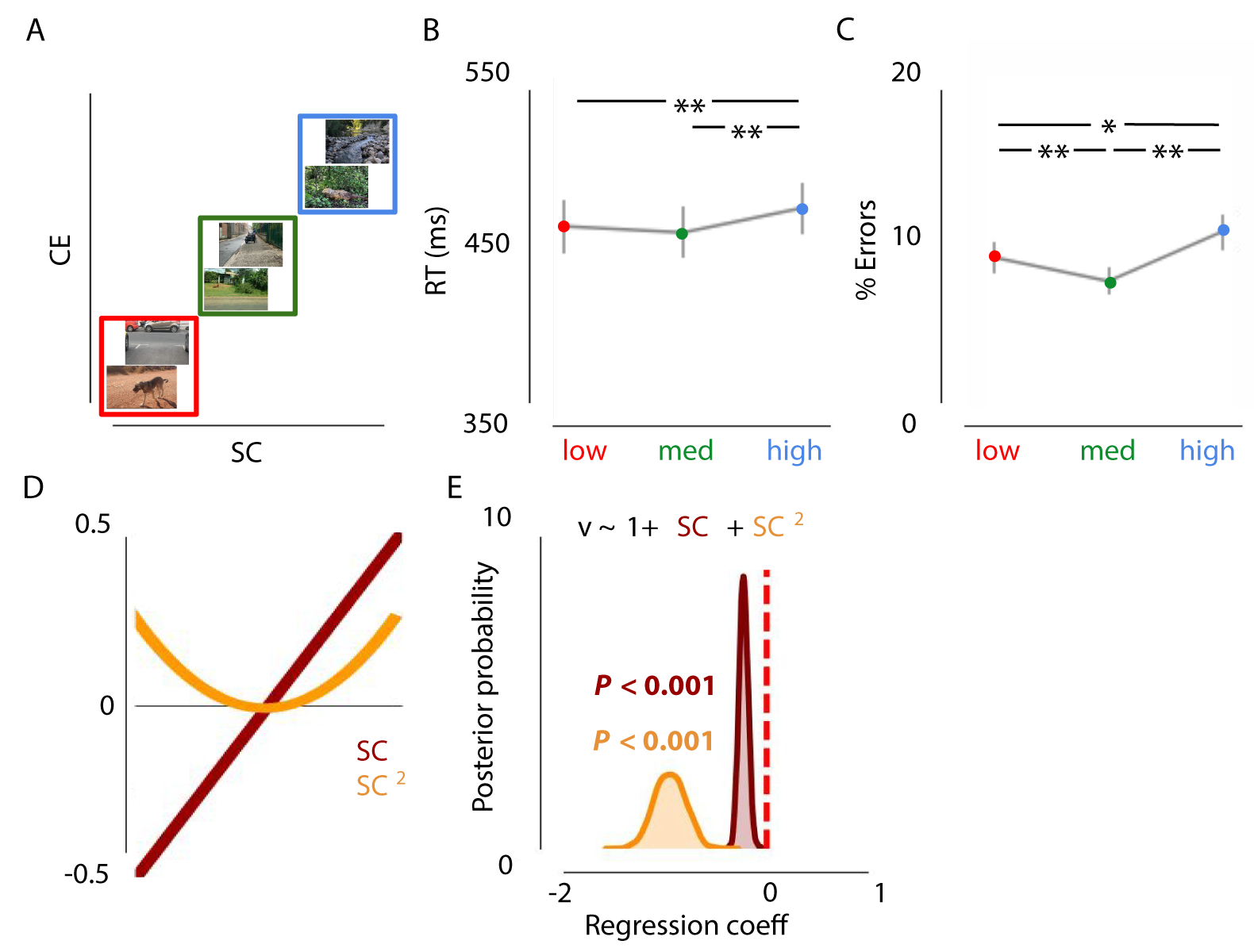
Figure 2.3: Effects of Spatial Coherence and Contrast Energy on animal vs. non-animal categorization. A) Examples of the stimuli used in experiment 1. Images varied both in SC and CE (red = low, green = medium, blue = high). B/C) Results of experiment 1 indicate worse performance for images with high SC/CE, as indicated by higher RTs and lowered accuracy. Error bars represent 1 SEM. * = p < .05, ** = p < .01, Bonferroni corrected. Task performance was best for medium SC/CE images. D) Schematic representation of the linear and quadratic terms included in the regression model. E) Low or high complexity (SC, strongly correlated to CE) was associated with a lower rate of evidence accumulation.

Thus, based on the reaction times and error rates, we were able to observe a decrease in performance for low and high complexity scenes. To understand this decrease in performance, we modeled the decision variables drift rate (speed of evidence accumulation) and response boundary (evidence requirements). Relative to the null model, the model in which only drift rate was affected by both \(SC\) and \(SC^2\) provided the best fit (\(\Delta\)DIC = -71.0, Figure 2.3), compared to models only including the centered or squared SC values and/or including a varying response boundary (see Supplementary section 2). That is, low and high SC were associated with a decreased drift rate (inverted U-shape; P < 0.001), as indicated by a negative shift in the posterior distribution. In other words, scene complexity influences the speed of information accumulation, resulting in higher reaction times and more errors for low and high complex scenes.

Experiment 2

Results experiment 2a

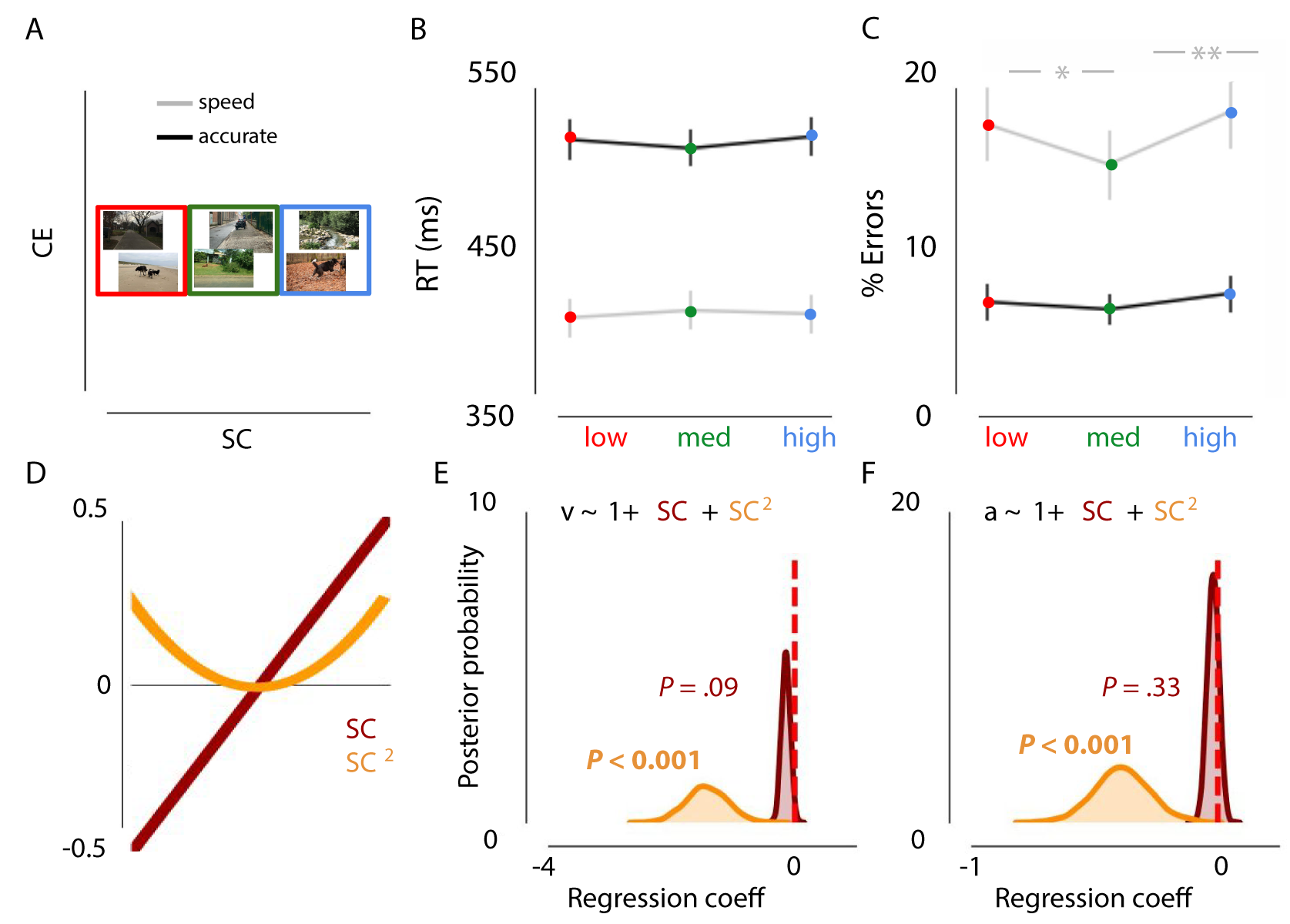
Figure 2.4: Effects of SC (controlling for Contrast Energy) on decision-making. A) Examples of the stimuli used in experiment 2a. Images only varied in SC, while CE was kept constant (red = low SC, green = medium SC, blue = high). B) Results showed no influence of SC on RT. C) Performance was most optimal for images with medium SC complexity in the speed condition, as indicated by a higher accuracy. Error bars represent 1 SEM. * = p < .05, ** = p < .01, Bonferroni corrected. D) Schematic representation of the linear and quadratic term included in the regression model. E/F) Negative shifts in the posterior distributions indicated that low or high complexity (SC) was associated with a lower rate of evidence accumulation and required less evidence to reach a decision (inverted U-shape).

One participant did not complete the experiment and was excluded from analyses. In contrast to experiment 1, the repeated-measures ANOVA on error rates and RTs showed, apart from the main effects of instruction and scene complexity, an interaction effect, F(42) = 4.351, p = 0.0189. Therefore, results were analyzed separately for “speed” and “accurate” trials to further understand how SC differentially impacts fast or accurate decision strategies.

The repeated-measures ANOVA revealed no main effect of SC on RTs for speeded or accurate trials (all p > 0.104). For error rates, there was a main effect of SC on speed trials, F(1, 44) = 9.189, p < .001, \(\eta^{2par}\) = .295. Participants made fewer errors for medium SC scenes compared to both low, t(22) = 3.294, p = 0.003 or high, t(22) = -4.346, p < .001 (Figure 2.4). Notably, SC had no effect on choice errors when participants were motivated to be accurate (p > .103)

Relative to the null model, the model in which drift rate and response boundary were affected by \(SC + SC^2\) provided the best fit (\(\Delta\)DIC = -21; Figure 2.4). As in experiment 1, low and high SC were associated with a decreased drift rate (inverted U-shape), as indicated by negative shifts in the posterior distribution (P < .001). Additionally, those scenes were associated with a decreased response boundary (P < .001; Figure 2.4), potentially to still allow for a timely response. Thus, SC influences the speed of information accumulation and the evidence requirements, resulting in more errors for low and high complex scenes when pressed for time.

Results experiment 2b

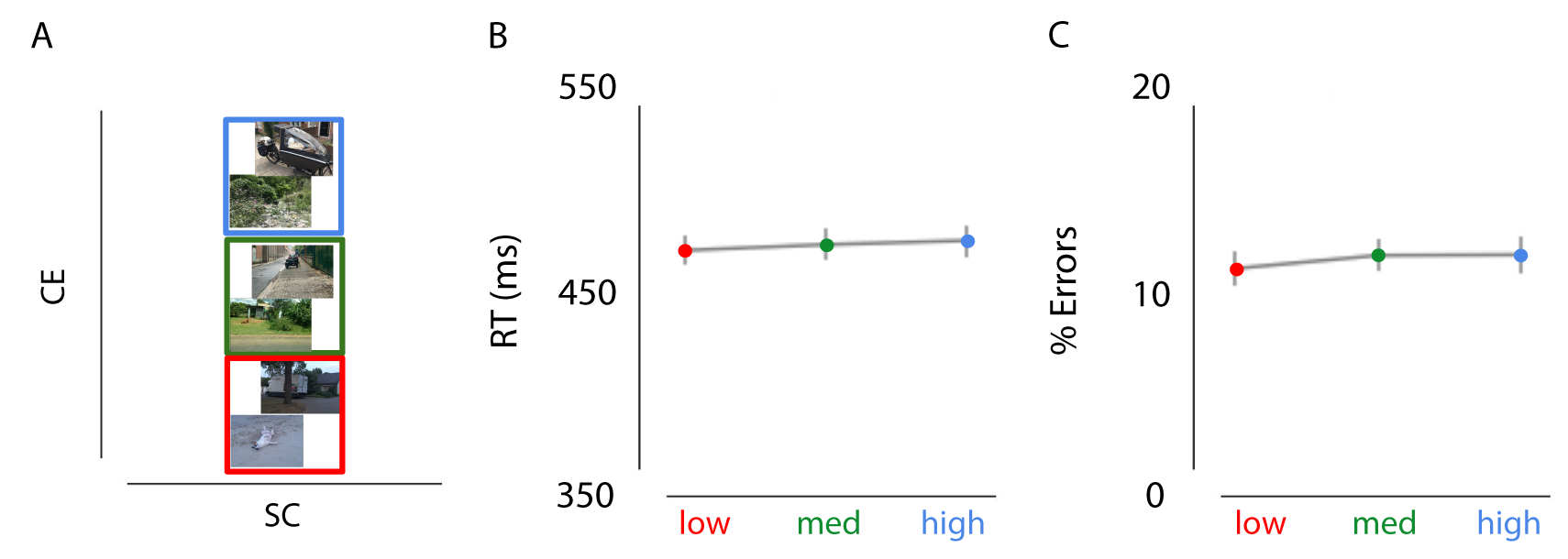
Figure 2.5: Effects of CE (controlling for Spatial Coherence) on decision-making. A) Examples of the stimuli used in experiment 2b. Images only varied in CE, while SC was kept constant (red = low CE, green = medium CE, blue = high CE). B/C) Results of experiment 2b showed no influence of CE on RT or percentage or errors.

Two participants were excluded because of excessive errors (>25%) or excessive omissions (>40%). A repeated-measures ANOVA with factors scene complexity (low, medium, high) and instruction (speed, accurate) revealed no interaction effects for RTs, F(48) = 0.093, p > 0.9, or errors, F(48) = 1.216, p > 0.3. Consistently, no main effect of CE was observed on RTs or errors when speeded and accurate trials were collapsed (Figure 2.5; all p > 0.306).

2.4 Discussion

This study systematically investigated the interaction between low-level statistics in natural scenes and perceptual decision-making processes. Results indicate that scene complexity, as indexed by two parameters (SC, CE), modulates perceptual decisions through the speed of information processing. Experiment 2a/b refined these observations by showing how the isolated manipulation of SC alone results in weaker yet comparable effects, whereas the manipulation of CE has no effect. By using natural stimuli, we show that task performance was best on medium complex images. Overall, these results show that very basic properties of our natural environment influence perceptual decision-making.

SC and CE together provide a compressed representation of scene complexity. While CE captures information about the amount and strength of edges in a scene, SC indexes higher-order correlations between them, giving an indication of the amount of clutter. In earlier work by Scholte et al. (2009) and Groen et al. (2013); Groen et al. (2016), differences in CE were shown to mainly influence the early part of the ERP, while SC effects arose later (up to 300 ms). In the current study, influences on perceptual decision-making seem to be mainly driven by SC. In experiment 1, when SC and CE were both manipulated, model selection indicated a better fit when changes in drift rate were related to SC (as compared to CE), and in experiment 2 only effects of SC were found. Still, there seems to be an additional influence of CE. The finding that there is no interaction between trial type and complexity condition in Experiment 1 indicates that even for trials in which there is ample time to process the image, scene complexity influences this process. Thus, while participants were faster and more susceptible to making errors when emphasizing speed (compared to accuracy), emphasis on speed or on accuracy did not change the magnitude of the scene complexity effect on both reaction times and errors. We interpret this as showing that the simultaneous manipulation of SC and CE leads to the strongest effects (as compared to experiment 2). In experiment 2a, in which CE was not manipulated, accuracy was decreased for low and high complexity trials only when participants were pressed for time. This suggests that for low and high complexity scenes, visual information processing might be too slow to produce correct responses, especially when participants are motivated to respond quickly and have lower evidence requirements in comparison to accurate instruction trials. In experiment 2a, low and high complexity scenes were, apart from drift rate, also associated with a lowered response boundary. Overall these results suggest that SC is weighed differently when manipulated in isolation. One explanation for the differences between experiment 1 and 2a could be the inherent correlation between the parameters in the real world, as isolating the influence of both parameters separately could have led to an ‘unnatural’ sub-selection. For this reason, we cannot attribute our results from experiment 2 exclusively to the scene statistics. Whether this is a robust effect should emerge from future research.

From previous studies, using artificial manipulation of stimulus quality, one would expect performance decreases for more complex scenes. For instance, the search slope of reaction times increases with the number of distractors in conjunction search (Wolfe, 1994) and degrading stimulus quality (via spatial filtering) reduces the rate of evidence accumulation (Jahfari et al., 2013). Intuitively ‘low’ SC scenes are easiest: those scenes are sparser and typically contain the most distinct figure-ground segmentation. Surprisingly, our results suggest a more complex pattern. In experiment 1 and 2a, performance was better on ‘medium’ than on ‘low’ scenes. Responses to natural scenes are often hard to predict from studies using artificial stimuli (Felsen & Dan, 2005) because the scenes do not contain simple isolated patterns. But why would scenes with medium SC/CE be processed more efficiently? We outline a number of possible reasons below.

First, it could be that scenes with medium complexity are most commonly encountered in daily life, and that the visual system has become tuned to the statistical regularities of medium scenes (Geisler & Diehl, 2003; Olshausen & Field, 1996), resulting in optimized visual processing.Secondly, it could be the degree to which object context facilitates the recognition process. In natural scenes, objects appearing in a familiar background are detected more accurately and quickly than objects in an unexpected environment (Davenport & Potter, 2004; Greene et al., 2015; Neider & Zelinsky, 2006). Here, most of the ‘low’ scenes contained little context because the backgrounds were, generally, homogeneous, providing no ‘cues’ about animal presence or absence. For ‘high’ images, on the other hand, there may have been too much distraction by spatially unorganized clutter, which does not offer useful cues for animal detection. Third, SC and CE could be related to certain object properties, such as animal size or centrality (the location of the animal in the scene). Additional HDDM analyses however indicated that SC contributed to perceptual decision-making independent of object size, whereas object centrality had no effects (Supplementary Figures S4-S6). Finally, SC/CE could be used as diagnostic information, serving as a building block towards estimating other relevant properties in a scene (e.g. scene clutter, naturalness). Since SC correlates with naturalness ratings (Groen et al., 2013) and, animals are potentially more strongly associated with natural environments, SC could be a diagnostic feature for the animal/non-animal discrimination task. Indeed, post-hoc evaluation of the responses in experiment 1 and 2a indicated a change in bias towards one of the response options (animal or non-animal), depending on the SC value of the scene. However, the pattern of errors, evaluated for animal and non-animal trials separately, was only partly consistent with a naturalness bias (Supplementary Figures S7 and S8). In the DDM, effects of a response bias can be explained either by changes in starting point (\(\Delta\)\(z\)) or by changes in drift rate (\(\Delta\)\(v\); (Mulder et al., 2012)) or the starting point of the drift rate. Additional modelling suggests that a potential response bias was not reflected in a change in the starting point, and the RT patterns for correct and incorrect trials in our dataset were more in line with a drift bias account (see Supplementary section 5). Crouzet & Serre (2011) have shown that low-level image properties such as SC and CE can relate to human performance in an animal detection task. When they trained a classifier to distinguish between animal/non-animal images based on the Weibull parameters (\(\beta\) and \(\gamma\)), classification performance was above chance, but relatively poor compared to alternative models which included more complex visual features, including oriented contrast (V1-like features) and combinations of oriented linear filter responses (mid-level and higher level features). Moreover, the least animal-like stimuli corresponded to more complex backgrounds, while our analyses of response bias (see Supplementary section 4) suggest the opposite pattern. This suggests that the relation between SC, naturalness and animal detection is not trivial and can vary with stimulus set or image database. Here, we carefully selected images to capture a broad range of CE and SC values, and ensured that animal presence was balanced within each condition. Therefore we believe that the current study is a more sensitive test of effects of low-level contrast statistics on perceptual discrimination than previous post-hoc assessments.

In conclusion, the current study provides clear evidence that SC and CE influence perceptual decision-making in an animal detection task. We propose that, because SC and CE could be plausibly computed in early stages of visual processing, they could indicate the need for more cautious or elaborate processing by providing the system with a global measure of scene complexity (Groen, Jahfari, et al., 2018). Future studies should pinpoint whether this effect is based on the computation of SC and CE directly, as a general measure of complexity, or indirectly, as diagnostic information to estimate other task-relevant scene properties. Given that the rate of evidence accumulation depends on the complexity of the scene, this complexity-dependent adaptation could be reflected in the amount of evidence that is considered sufficient for generating a response. This adaptation, or flexible processing, can help to calibrate the decision process to maximize the goal at hand (e.g. to be accurate or quick).

2.5 Supplement to Chapter 2

2.5.1 1. Computation of SC and CE

The following section describes the main computational steps. The code to run the model on an arbitrary input image is available on Github.

2.5.1.1 Natural image statistics: local contrast distribution regularities.

Natural images exhibit much statistical regularity, one of which is present in the distribution of local contrast values. It has been observed (Simoncelli, 1999; Geusebroek and Smeulders, 2002, 2005) that properties that are inherent to natural images, such as spatial fragmentation (generated by the edges between the objects in the scene) and local correlations (due to edges belonging to objects in the image) results in contrast distributions that range between power law and Gaussian shapes, and therefore conform to a Weibull distribution. This regularity (systematic variation in the contrast distribution of natural images) can therefore be adequately captured by fitting a Weibull function of the following form:

\(p(f) = c e^{\frac{(f-\mu)} {\beta} \gamma}\)

Where \(c\) is a normalization constant that transforms the frequency distribution into a probability distribution. The parameter \(\mu\), denoting the origin of the contrast distribution, is generally close to zero for natural images. We normalize out this parameter by subtracting the smallest contrast value from the contrast data, leaving two free parameters per image, \(\beta\) (beta) and \(\gamma\) (gamma), that represent the scale (beta) and shape (gamma) of the distribution (Geusebroek & Smeulders, 2002, 2005). Beta varies with the range of contrast strengths present in the image, whereas gamma varies with the degree of correlation between contrasts.

2.5.1.2 LGN model of local contrast statistics: contrast energy and spatial coherence.

In previous work, we found that the beta and gamma parameters of the Weibull distribution can be approximated in a physiologically plausible way by summarizing responses of receptive field models to local contrast (Scholte et al., 2009). Specifically, summing simulated receptive field responses from a model of the parvocellular and magnocellular pathways in the LGN led to accurate approximations of beta and gamma, respectively. In subsequent papers (Groen et al., 2013, 2017) an improved version of this model was presented in which contrast was computed at multiple spatial scales and the LGN approximations were estimated not via summation but by averaging the local parvocellular responses (for beta) and by averaging and divisively normalizing the magnocellular responses for gamma (mean divided by standard deviation). To distinguish the Weibull fitted parameters from the LGN approximations, the LGN-approximated beta value was defined as Contrast Energy (CE) and the LGN-approximated value of gamma as spatial coherence (SC). These modifications, as well as specific parameter settings in the model, were determined based on comparisons between the Weibull fitted values and the CE/SC values, as well as model fits to EEG responses, in separate, previously published image sets (Ghebreab et al., 2009, Scholte et al., 2009). We outline the main computational steps of the model below:

2.5.1.3 Main computational steps of the model

Step 1: RGB to color opponent space. For each image, the input RGB values were converted to opponent color space using the Gaussian color model described in (Geusebroek, Van den Boomgaard, Smeulders & Geerts, 2001), yielding 3 opponent color values per pixel (grayscale, blue-yellow, red-green; Koenderink, Van De Grind & Bouman, 1972).

Step 2: Multi-scale local contrast detection. Each color opponent layer was convolved with isotropic exponential filters (Zhu and Mumford, 1997) at five octave scales (Croner and Kaplan, 1995). Two separate filter sets were used: smaller filter sizes (0.12, 0.24, 0.48, 0.96, and 1.92 degrees) for CE and larger filter sizes (0.16, 0.32, 0.64, 1.28, and 2.56 degrees) for SC (Ghebreab et al., 2009). Following the LGN suppressive field approach (Bonin et al., 2005), all filter responses were rectified and divisively normalized.

Step 3: Scale selection. Per parameter (CE or SC) and color-opponent layer, one filter response was selected for each image location from their respective filter set using minimum reliable scale selection (Elder and Zucker, 1998). In this MIN approach, the smallest filter size that yields an above-threshold response is preferred over other filter sizes. Filter-specific noise thresholds were determined from a separate image set (Corel database) (Ghebreab et al., 2009).

Step 4: Spatial pooling. Applying the selected filters for each image location results in two contrast magnitude maps: one highlighting detailed edges (from the set of smaller filter sizes, for CE) and the other more coarse edges (from the set of larger filter sizes, for SC) per color opponent-layer. To simulate the different visual field coverage of parvo- and magnocellular pathways, a different amount of visual space was taken into account for each parameter in the spatial pooling step. For CE, the central 1.5 degrees of the visual field was used, whereas for SC, 5 degrees of visual field was used. Finally, the estimated parameter values were averaged across color-opponent layers resulting in a single CE and SC value per image.

2.5.2 2. HDDM model comparison and convergence

First, we evaluated five models in which drift rate (\(v\)) and boundary (\(a\)) were either fixed or varied across trial type (speed, accurate) and/or scene complexity (low, medium, high).

Table 2.1: HDDM model fits to determine whether varying across scene complexity was justified to account for the data. We evaluated five models in which drift rate (v) and boundary (a) were either fixed or varied across trial type (speed, accurate) and/or scene complexity (low, medium, high).

	drift rate (v)	boundary (a)	DIC - exp 1	DIC - exp 2a	DIC - exp 2b
model 0	-	-	-11453.46	-8545.74	-7240.21
model 1	-	instruction	-14857.92	-11971.86	-10109.50
model 2	complexity	instruction	-14885.64	-11939.36	-10064.76
model 3	-	instruction, complexity	-14792.76	-11929.10	-10032.79
model 4	complexity	instruction, complexity	-14926.04	-11999.62	-10060.99

Then, to assess the trial-by-trial relationship between scene complexity and drift rate (v) and boundary separation (a), we fitted eighteen alternative regression models.

Table 2.2: HDDM Regression models. Drift rate \(v\) and boundary \(a\) were either allowed to vary across scene complexity (indexed by SC or CE) or fixed. Both linear models (SC/CE centered around zero), and second-order polynomial models (quadratic) were fitted to examine whether the relationship was curvilinear (e.g. followed an inverted U-shape).

	drift rate (v)	boundary (a)	both (\(v,a\))
\(SC\)	model 1	model 2	model 3
\(SC^2\)	model 4	model 5	model 6
\(SC+ SC^{2}\)	model 7	model 8	model 9
\(CE\)	model 10	model 11	model 12
\(CE^{2}\)	model 13	model 14	model 15
\(CE+ CE^{2}\)	model 16	model 17	model 18

Table 2.3: Means of the posterior distributions.

parameter	Experiment 1	Experiment 2a
\(t\)	0.18	0.23
\(z\)	0.27	0.29
\(v\_Intercept\)	3.69	3.16
\(v\_SC\)	0.23	-0.14
\(v\_SC^{2}\)	-0.96	-1.43
\(a\_Intercept(Ac)\)	1.93	1.85
\(a\_Intercept(Sp)\)	1.46	1.47
\(a\_SC\)	-	-0.02
\(a\_SC^{2}\)	-	-0.39

2.5.3 3. HDDM analyses incorporating contextual factors

The following section describes the methods for the additional analyses to evaluate potential contextual factors that could correlate with SC and limit the detection task. Specifically, we parameterized two characteristics, object size and centrality. We have focused on these two factors, because just like CE and SC, they were image-computable, i.e. they could be derived by performing calculations on the pixels in the image.

2.5.3.1 Computing contextual factors

Object size was computed by taking the percentage of the image that was covered by the animal (manually segmented). Object centrality was computed by taking the distance in pixels from the center of mass (CoM) of the animal (computed by interpreting the image as a 2D probability distribution) to the center of the screen (see Supplementary Figure 2.6).

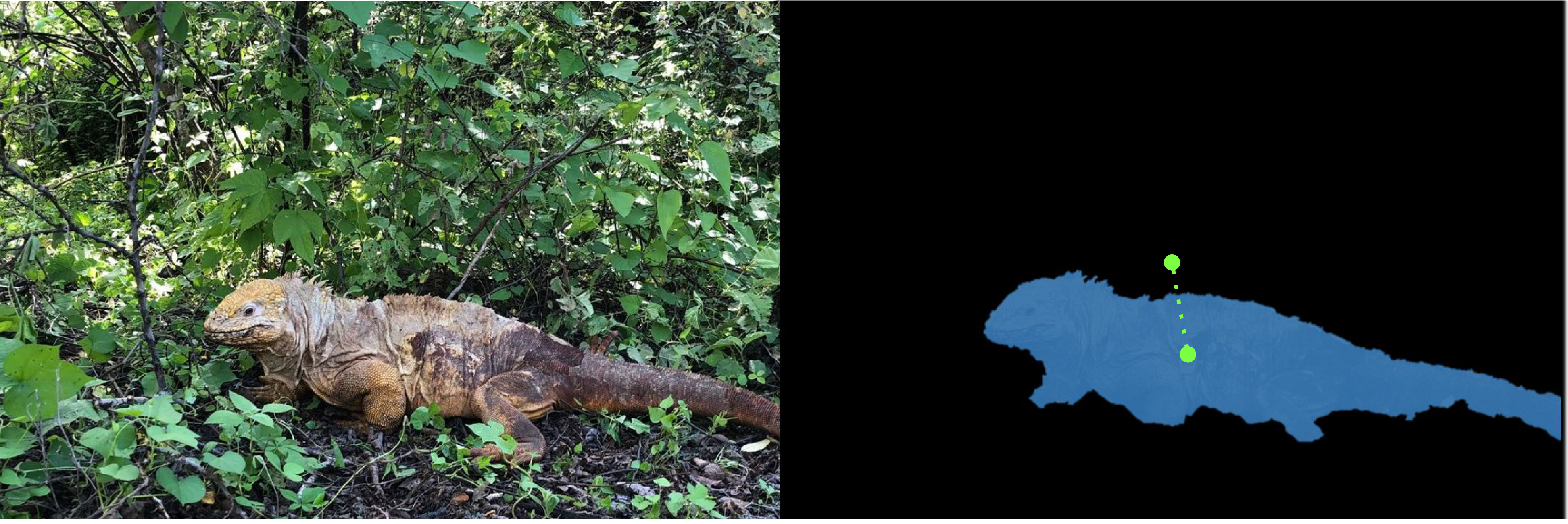
Figure 2.6: Example of computing object (animal) coverage and centrality. Object size was computed by taking the percentage of the image that was covered by the animal (manually segmented). Object centrality was computed by taking the distance from the center of mass (CoM) of the animal to the center of the screen (length of green dotted line, in pixels).

2.5.3.2 Evaluating the relationship with SC and CE

There was no correlation between SC or CE and object coverage (experiment 1; SC: \(r\) = 0.018; CE: \(r\) = 0.025) or centrality (SC: \(r\) = -0.13; CE: \(r\) = -0.09). To evaluate whether SC explains unique variance after accounting for these properties, we included both variables in our HDDM regression analysis, alongside SC.

For experiment 1, results showed an influence of object size (coverage) on the drift rate, with a higher drift rate for images with larger animals as indicated by a positive shift in the posterior distribution (Supplementary Figure S2; P < .001). For object centrality, however, we found no effect, and inspection of this variable indicated a low variability: most animals were located quite central. In experiment 2a, as in experiment 1, larger animals were associated with a higher drift rate (Supplementary Figure S3; P < .001). Most importantly, for both experiments, the effect of SC remained. This indicates that, even though object size has an influence on the rate of evidence accumulation, SC continues to explain unique variance in the speed of information processing. In other words, SC contributes to perceptual decision-making independent of object size, whereas object centrality has no effects.

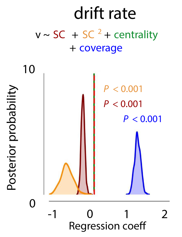
Figure 2.7: Effects of SC/CE (experiment 1) on drift rate, accounting for object size and centrality. Bigger animals were associated with a higher rate of evidence accumulation. The effects of SC+SC2 remained, indicating that, even though object size has an influence on the rate of evidence accumulation, SC continues to explain unique variance in the speed of information processing.

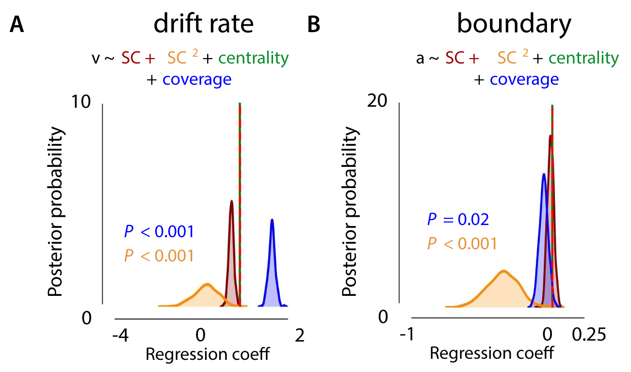
Figure 2.8: Effects of SC (experiment 2a) on drift rate and response boundary, accounting for object size and centrality. Bigger animals were associated with a higher rate of evidence accumulation. Again, the effect of SC2 remained, indicating that even though object size has an influence on the rate of evidence accumulation, SC continues to explain unique variance in the speed of information processing.

Full description and code definitions can be found on Github

2.5.4 4. Behavioral analysis evaluating animal/non-animal bias

To investigate whether participants’ response bias (towards animal or non-animal) differed with scene complexity, we computed the % animal choices for each participant. Differences between the three conditions (low, med, high) were statistically evaluated using a repeated-measures ANOVA.

For experiment 1, results indicated, apart from a general bias towards the non-animal option (animal choice < 50% for all conditions), that the % animal-responses increases with scene complexity, F(36) = 9.76, p < 0.001, \(\eta^{2par}\) = .351 (Supplementary Figure S4). Participants chose ‘animal’ more often in the high and medium complexity scenes as compared to low, t(18) = -5.104, p < .001; t(18) = -2.698, p = .044 (Bonferroni corrected). Similar effects were found for experiment 2a (Supplementary Figure S5). There, the percentage of animal responses increased with SC, F(44) = 6.63, p = 0.003, \(\eta^{2par}\) = .232. Participants chose ‘animal’ more often in the high scenes as compared to low, t(22) = -3.365, p = .008 (Bonferroni corrected). In the current experiment, half of the trials in each condition contained an animal. Therefore, this response bias towards animal or non-animal trials can result in an increase in errors in the low and high condition. Analysis of the error rates separately for animal and non-animal trials, indicated for both experiment 1 and experiment 2a that most errors in the low condition were made for animal-trials. In those trials, participants thus seem to ‘miss’ the animal more often. Errors in high scenes, however, were seemingly not caused by the response bias: while participants reported more animals on non-animal trials (compared to low and medium), they made as many errors on animal trials.

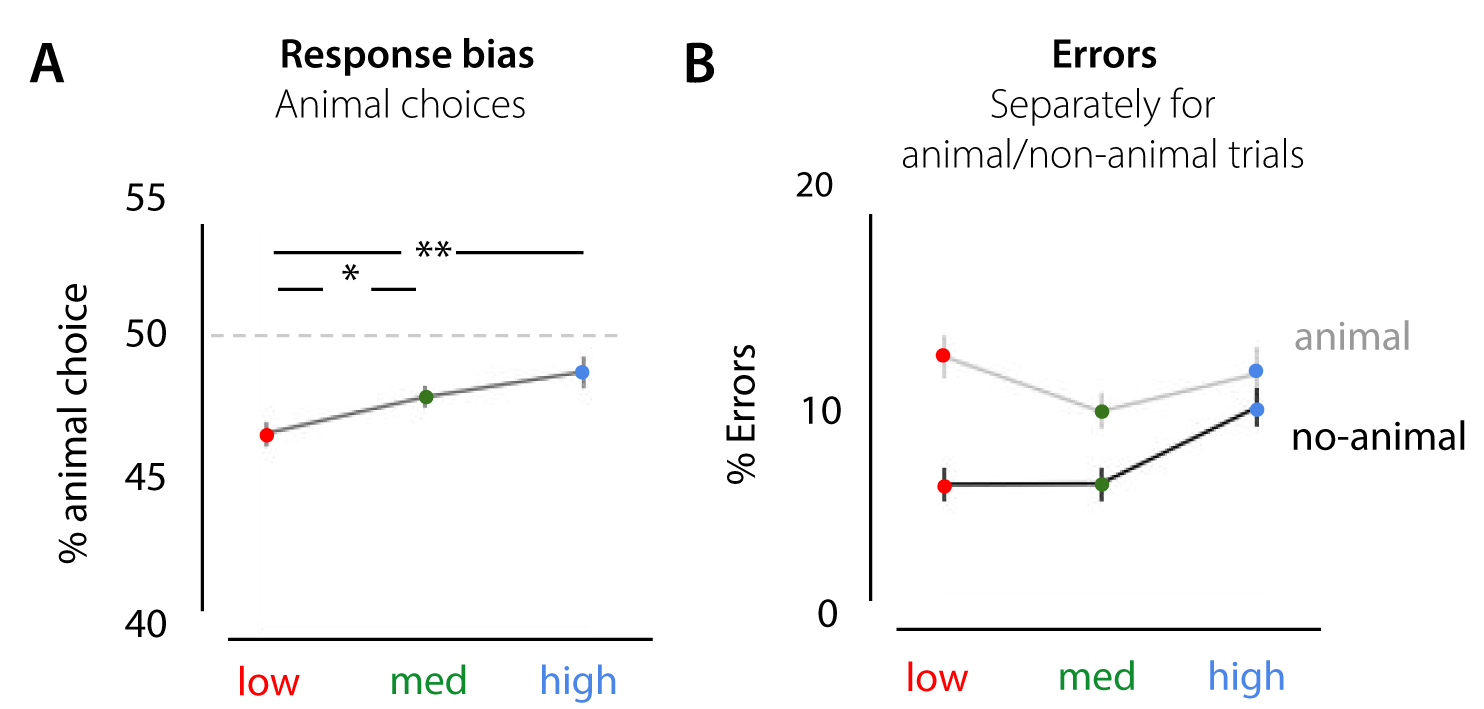
Figure 2.9: Response bias effects in experiment 1. A) apart from a general bias towards the non-animal option (animal choice < 50% for all conditions), the % animal-responses increased with scene complexity. B) percentage of errors from experiment 1, separately for animal and non-animal trials.

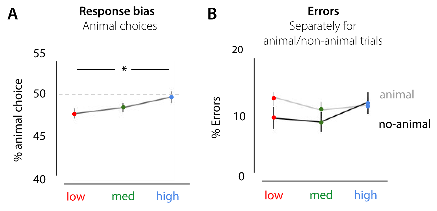
Figure 2.10: Effects of SC on animal/non-animal responses in experiment 2a. A) Similar to experiment 1, the % animal-responses increased with SC. B) Percentage of errors from experiment 2a, plotted separately for animal and non-animal trials.

2.5.5 5. HDDM Regression analyses evaluating response bias effects

Following Supplementary section 4, to assess whether SC biases the response (towards animal or non-animal) reflected in changes in the starting point, we fitted several HDDMRegressor models: 1. one model in which we estimate only the response bias z for every complexity condition (low, med, high), such that the bias for animal stimuli is z and the bias for non-animal stimuli is 1-z (z = 0.5 for unbiased decisions in HDDM. 2. one model in which we estimate both v and z. This way, we could measure response-bias (in favor of animal or non-animal) and drift rate for the three conditions (low, med, high) while assuming the same drift rate for both stimuli. 3. one model in which we estimate v, z and a for every complexity condition. 4. one model in which we estimate v, z and a for every complexity condition and, using the depends_on key argument, two intercepts for a (speed, accurate) 5. same model as the previous model (4), now using ‘medium’ as the intercept for z

However, with the properties of our observations and design, models defined in this way do not converge, which makes the interpretation of the parameters uninformative. The traces are non-stationary, and the autocorrelation is high. The histograms look serrated. Full description and code definitions can be found on Github

Then, we fit one model using HDDMStimCoding, in which we estimate \(v\), \(z\) for every complexity condition, and a for every complexity condition + speed/accuracy instruction. This model converges. As shown in the figure (Supplementary figure S9) below, the obtained posteriors for \(z\) do not differ across our low, med, or high condition. Hence, this evaluation shows no effect of condition (low, med, high) on \(z\) when it is allowed to vary.

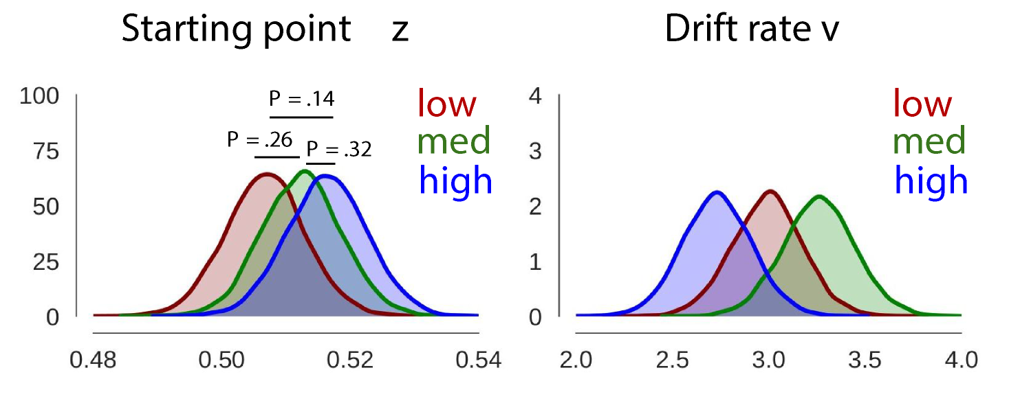
Figure 2.11: Using HDDMStimCoding to evaluate potential biases towards animal/non-animal across the different conditions for the data obtained in experiment 1.

In the DDM, effects of a response bias can be explained either by changes in starting point (\(\Delta\)\(z\)) or by changes in drift rate (\(\Delta\)\(v\); Mulder, Wagenmakers, Ratcliff, Boekel & Forstmann, 2012)) or the starting point of the drift rate. Additional modeling suggests that a potential response bias was not reflected in a change in the starting point and the RT patterns for correct and incorrect trials in our dataset were more in line with a drift bias account:

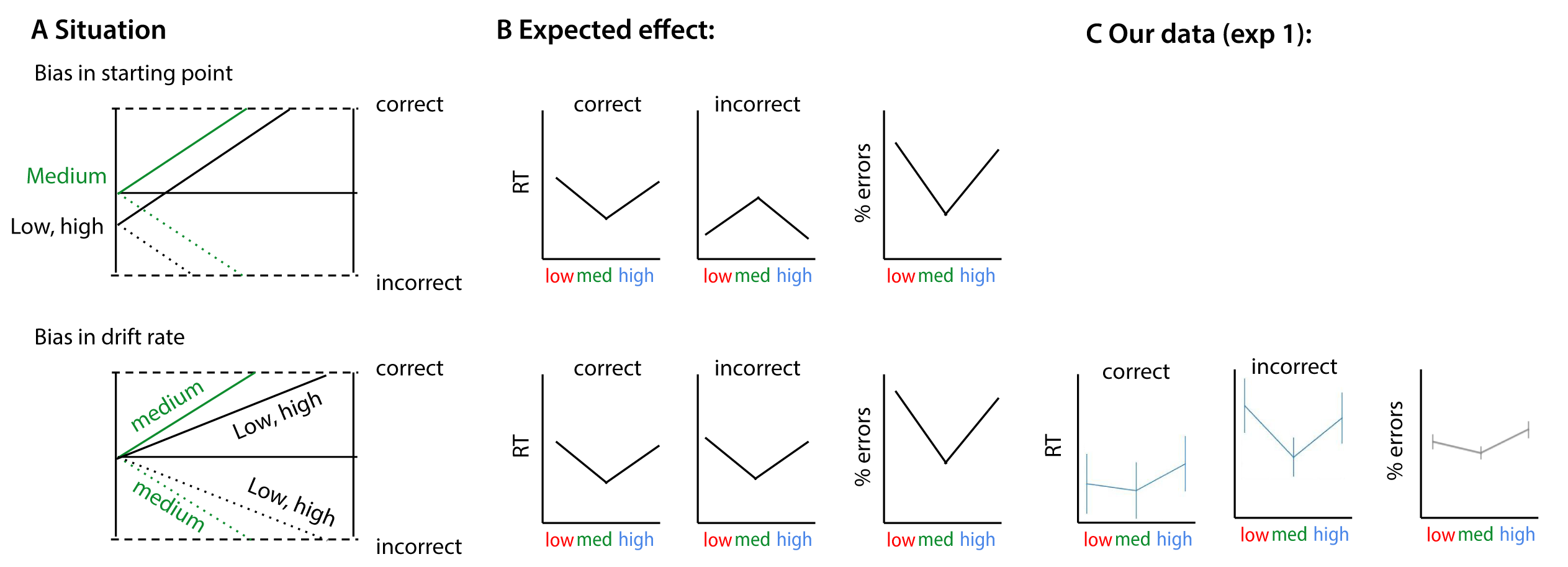
Figure 2.12: Possible effects of bias on choice behavior (following figure 2 from Mulder et al. (2012)). A) Effects of bias explained by the drift-diffusion model. When prior information is invalid (‘low’, ‘high’) for the choice at hand, subjects will have slower and less correct choices compared with choices where no information is provided (neutral, ‘medium’). These effects can be explained by changes in the starting point or the drift rate of the accumulation process. B) Both accounts have different effects on RT and accuracy data. C) The data from our current experiment is more in line with a drift rate account of response bias.

References

Brady, N., & Field, D. J. (2000). Local contrast in natural images: Normalisation and coding efficiency. Perception, 29(9), 1041–1055.

Crouzet, S. M., & Serre, T. (2011). What are the visual features underlying rapid object recognition? Front. Psychol., 2, 326.

Davenport, J. L., & Potter, M. C. (2004). Scene consistency in object and background perception. Psychol. Sci., 15(8), 559–564.

Deng, J. D. J., Dong, W. D. W., Socher, R., Li, L.-J. L. L.-J., Li, K. L. K., & Fei-Fei, L. F.-F. L. (2009). ImageNet: A large-scale hierarchical image database. 2009 IEEE Conference on Computer Vision and Pattern Recognition, 2–9.

Felsen, G., & Dan, Y. (2005). A natural approach to studying vision. Nat. Neurosci., 8(12), 1643–1646.

Geisler, W. S., & Diehl, R. L. (2003). A bayesian approach to the evolution of perceptual and cognitive systems. Cogn. Sci., 27(3), 379–402.

Ghebreab, S., Scholte, S., Lamme, V., & Smeulders, A. (2009). A biologically plausible model for rapid natural scene identification. Adv. Neural Inf. Process. Syst., 629–637.

Gold, J. I., & Shadlen, M. N. (2007). The neural basis of decision making. Annu. Rev. Neurosci., 30, 535–574.

Greene, M. R., Botros, A. P., Beck, D. M., & Fei-Fei, L. (2015). What you see is what you expect: Rapid scene understanding benefits from prior experience. Atten. Percept. Psychophys., 1239–1251.

Greene, M. R., & Oliva, A. (2009a). Recognition of natural scenes from global properties: Seeing the forest without representing the trees. Cogn. Psychol., 58(2), 137–176.

Greene, M. R., & Oliva, A. (2009b). The briefest of glances: The time course of natural scene understanding. Psychol. Sci., 20(4), 464–472.

Groen, I. I. A., Ghebreab, S., Lamme, V. A. F., & Scholte, H. S. (2010). The role of weibull image statistics in rapid object detection in natural scenes. J. Vis., 10(7), 992–992.

Groen, I. I. A., Ghebreab, S., Lamme, V. A. F., & Scholte, H. S. (2016). The time course of natural scene perception with reduced attention. J. Neurophysiol., 115(2), 931–946.

Groen, I. I. A., Ghebreab, S., Prins, H., Lamme, V. A. F., & Scholte, H. S. (2013). From image statistics to scene gist: Evoked neural activity reveals transition from Low-Level natural image structure to scene category. Journal of Neuroscience, 33(48), 18814–18824.

Groen, I. I. A., Jahfari, S., Seijdel, N., Ghebreab, S., Lamme, V. A., & Scholte, H. S. (2018). Scene complexity modulates degree of feedback activity during object detection in natural scenes. PLoS Computational Biology, 14(12), e1006690.

Heekeren, H. R., Marrett, S., & Ungerleider, L. G. (2008). The neural systems that mediate human perceptual decision making. Nat. Rev. Neurosci., 9(6), 467–479.

Jahfari, S., Ridderinkhof, K. R., & Scholte, H. S. (2013). Spatial frequency information modulates response inhibition and decision-making processes. PLoS One, 8(10), e76467.

Jahfari, S., Waldorp, L., Ridderinkhof, K. R., & Scholte, H. S. (2015). Visual information shapes the dynamics of corticobasal ganglia pathways during response selection and inhibition. J. Cogn. Neurosci., 1344–1359.

Jegou, H., Douze, M., & Schmid, C. (2008). Hamming embedding and weak geometric consistency for large scale image search. European Conference on Computer Vision, 5302 LNCS(PART 1), 304–317.

Malcolm, G. L., Groen, I. I. A., & Baker, C. I. (2016). Making sense of real-world scenes. Trends Cogn. Sci., 20(11), 843–856.

Mulder, M. J., Wagenmakers, E.-J., Ratcliff, R., Boekel, W., & Forstmann, B. U. (2012). Bias in the brain: A diffusion model analysis of prior probability and potential payoff. J. Neurosci., 32(7), 2335–2343.

Neider, M. B., & Zelinsky, G. J. (2006). Scene context guides eye movements during visual search. Vision Res., 46(5), 614–621.

Oliva, A., & Torralba, A. (2001). Modeling the shape of the scene: A holistic representation of the spatial envelope. Int. J. Comput. Vis., 42(3), 145–175.

Olmos, A., & Kingdom, F. A. A. (2004). A biologically inspired algorithm for the recovery of shading and reflectance images. Perception, 33(12), 1463–1473.

Olshausen, B. A., & Field, D. J. (1996). Natural image statistics and efficient coding. Network: Computation in Neural Systems, 7(2), 333–339.

Opelt, A., Pinz, A., Fussenegger, M., & Auer, P. (2006). Generic object recognition with boosting. IEEE Trans. Pattern Anal. Mach. Intell., 28(3), 416–431.

Ratcliff, R. (2014). Measuring psychometric functions with the diffusion model. J. Exp. Psychol. Hum. Percept. Perform., 40(2), 870.

Ratcliff, R., & Childers, R. (2015). Individual differences and fitting methods for the Two-Choice diffusion model of decision making. Decision (Wash D C ), 2015.

Ratcliff, R., & McKoon, G. (2008). The diffusion decision model: Theory and data for Two-Choice decision tasks. Neural Comput., 29(6), 997–1003.

Rosenholtz, R., Huang, J., Raj, A., Balas, B. J., & Ilie, L. (2012). A summary statistic representation in peripheral vision explains visual search. J. Vis., 12(4).

Scholte, H. S., Ghebreab, S., Waldorp, L., Smeulders, A. W. M., & Lamme, V. A. F. (2009). Brain responses strongly correlate with weibull image statistics when processing natural images. J. Vis., 9(4), 29–29.

Spiegelhalter, D. J., Best, N. G., Carlin, B. P., & Van Der Linde, A. (2002). Bayesian measures of model complexity and fit. J. R. Stat. Soc. Series B Stat. Methodol., 64(4), 583–639.

Thorpe, S., Fize, D., & Marlot, C. (1996). Speed of processing in the human visual system. Nature, 381(6582), 520.

Wiecki, T. V., Sofer, I., & Frank, M. J. (2013). HDDM: Hierarchical bayesian estimation of the drift-diffusion model in python. Front. Neuroinform., 7, 14.

Wolfe, J. M. (1994). Guided search 2.0 a revised model of visual search. Psychon. Bull. Rev., 1(2), 202–238.